Introduction

In this vignette, we will estimate individual genetic distances from SNP data. It is useful when you have individual genotype data and you don’t know the populations.

Assumptions

We will use non-evolutionary genetic distances, i.e. not based on Hardy-Weinberg assumptions: free from assumptions.

Data

The dataset used for those analysis concerns the plant: lodgepole pine (Pinus contorta, Pinaceae). You can have more information on this data set and the species on the web site of A. Eckert: (http://eckertdata.blogspot.fr/). But here the dataset is used as a test dataset with no idea of interpreting the results in a biological way. We will work on a subset of the dataset to make the calculations faster.

The data are stored in a text file (genotype = AA). We will import the dataset in R as a data frame, and then convert the SNP data file into genind objects.

The dataset “Master_Pinus_data_genotype.txt” can be downloaded here.

The text file is a matrix of (550 rows x 3086 columns). It contains 4 extra columns: first column is the label of the individuals, the three other are description of the region, all the other columns are for the genotypes as (AA or AT…).

When you import the data into R, the data file needs to be in your working directory, or adjust the path in the read.table() invocation below accordingly.

Mydata <- read.table("Master_Pinus_data_genotype.txt", header = TRUE, check.names = FALSE)   
dim(Mydata)

## [1]  550 3086

ind <- as.character(Mydata$tree_id) # individual labels 
population <- as.character(Mydata$state) # population labels
county <- Mydata$county 
dim(Mydata) # 550 individuals x 3082 SNPs

## [1]  550 3086

Resources/Packages required

Loading the required packages:

library("poppr")
library("pegas")
library("ape")
library("adegenet")
library("ade4")

Analysis

Section 1: Convert the data

To work with the data, we need to convert the R object returned by read.table() to a genind object. To achieve this, we create a matrix with only genotypes, and keep only a subset of the first 100 SNP loci (to make calculations faster). The result can then be converted to a genind object (for the package adegenet). The genind object can then easily be converted into loci objects (package pegas) (i.e. Mydata2)

locus <- Mydata[, -c(1, 2, 3, 4, 105:ncol(Mydata))] 
Mydata1 <- df2genind(locus, ploidy = 2, ind.names = ind, pop = population, sep="")
Mydata1

## /// GENIND OBJECT /////////
## 
##  // 550 individuals; 100 loci; 200 alleles; size: 530.6 Kb
## 
##  // Basic content
##    @tab:  550 x 200 matrix of allele counts
##    @loc.n.all: number of alleles per locus (range: 2-2)
##    @loc.fac: locus factor for the 200 columns of @tab
##    @all.names: list of allele names for each locus
##    @ploidy: ploidy of each individual  (range: 2-2)
##    @type:  codom
##    @call: df2genind(X = locus, sep = "", ind.names = ind, pop = population, 
##     ploidy = 2)
## 
##  // Optional content
##    @pop: population of each individual (group size range: 4-177)

Mydata2 <-genind2loci(Mydata1)

Section 2. Individual genetic distance: euclidean distance (`dist` {adegenet})

The unit of the observation is the individuals.

550 genotypes
100 binary SNPs
Ploidy : 2

The analysis is applied on allele frequency within individuals as represented in the genind object. We can use the function dist() from adegenet which provides different options. We will use the euclidean distance among vector of allele frequencies.

distgenEUCL <- dist(Mydata1, method = "euclidean", diag = FALSE, upper = FALSE, p = 2)
hist(distgenEUCL)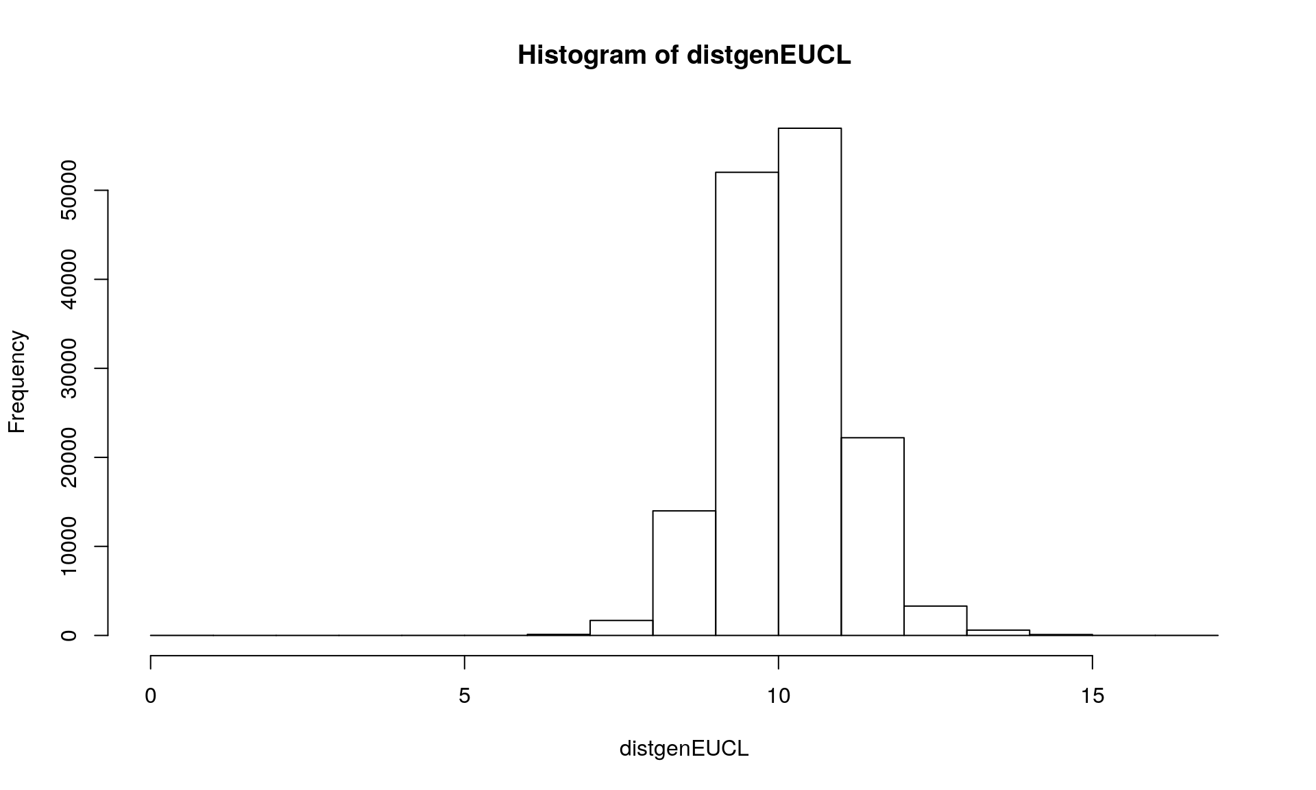

Section 3. Individual genetic distance: number of loci for which individuals differ (`dist.gene` {ape})

The option pairwise.deletion = FALSE in the command dist.gene() removes all loci with one missing values : you an see on the histogram that we get a maximum distance of 3 loci out of 100.

We can see that we get 98 loci with at least one sample missing. Then using the option pairwise.deletion = TRUE in the command dist.gene() allows you to keep loci with one missing value.

distgenDIFF <- dist.gene(Mydata2, method="pairwise", pairwise.deletion = FALSE, variance = FALSE)
hist(distgenDIFF)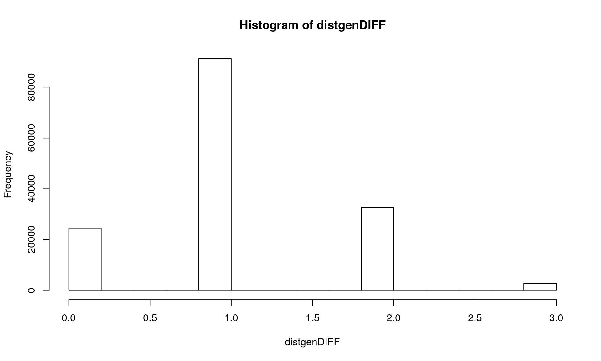

# Get percent missing data per population
missing_data <- info_table(Mydata1, type = "missing")
sum(missing_data["Total", 1:100] > 0)

## [1] 98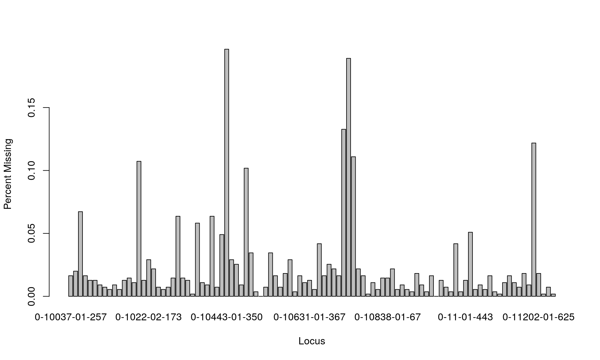

barplot(missing_data["Total", 1:100], xlab = "Locus", ylab = "Percent Missing")

distgenDIFF <- dist.gene(Mydata2, method="pairwise", pairwise.deletion = TRUE, variance = FALSE)
hist(distgenDIFF)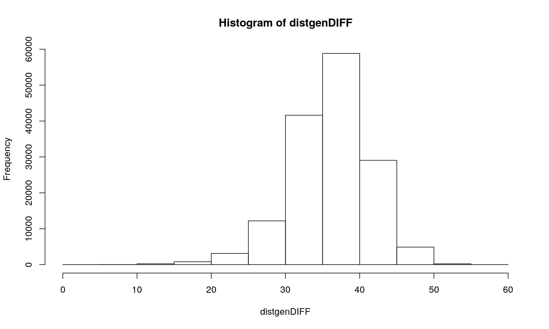

Section 4: number of allelic differences between two individuals (`diss.dist` {poppr})

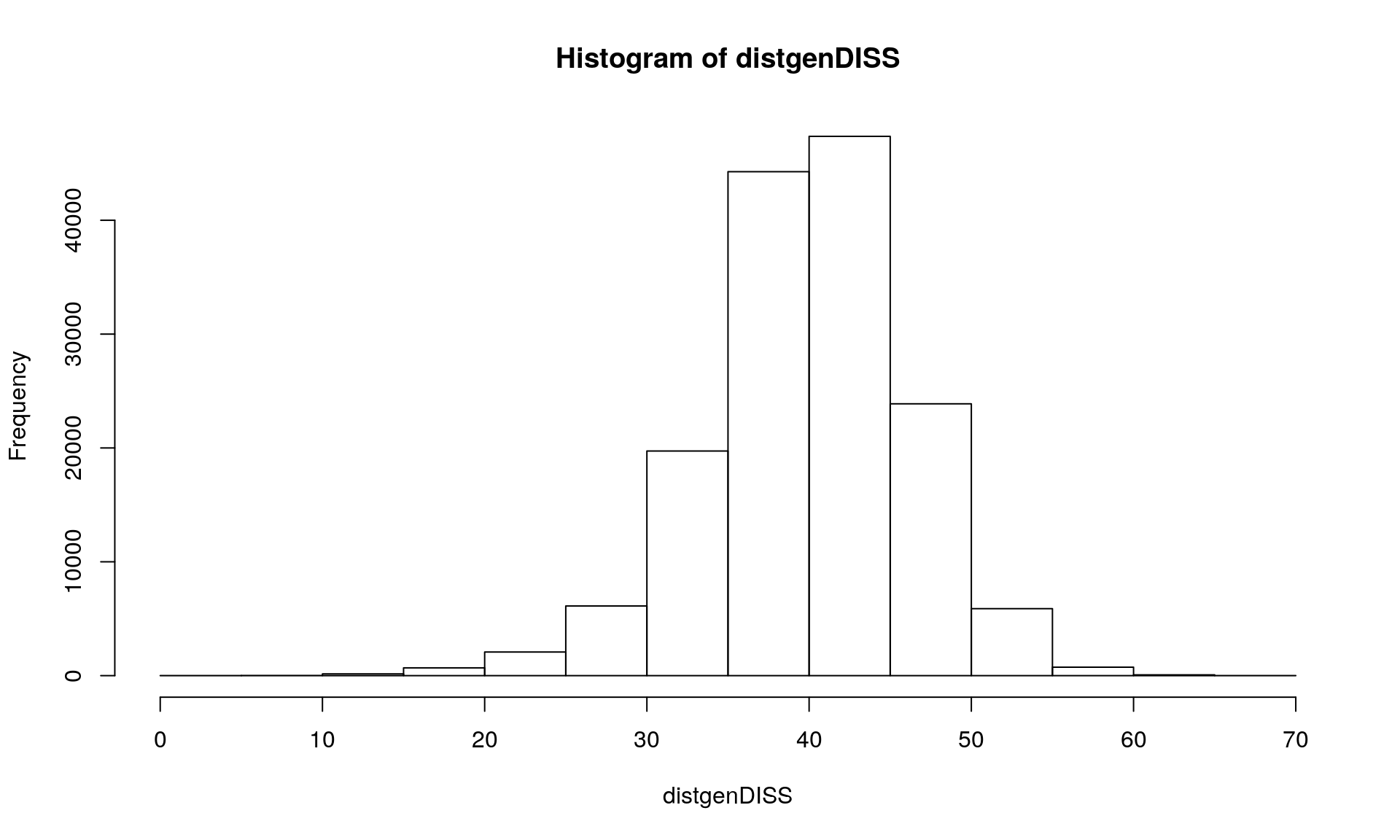
distgenDISS <- diss.dist(Mydata1, percent = FALSE, mat = FALSE)
hist(distgenDISS)

Section 5: Conclusions drawn from the analysis

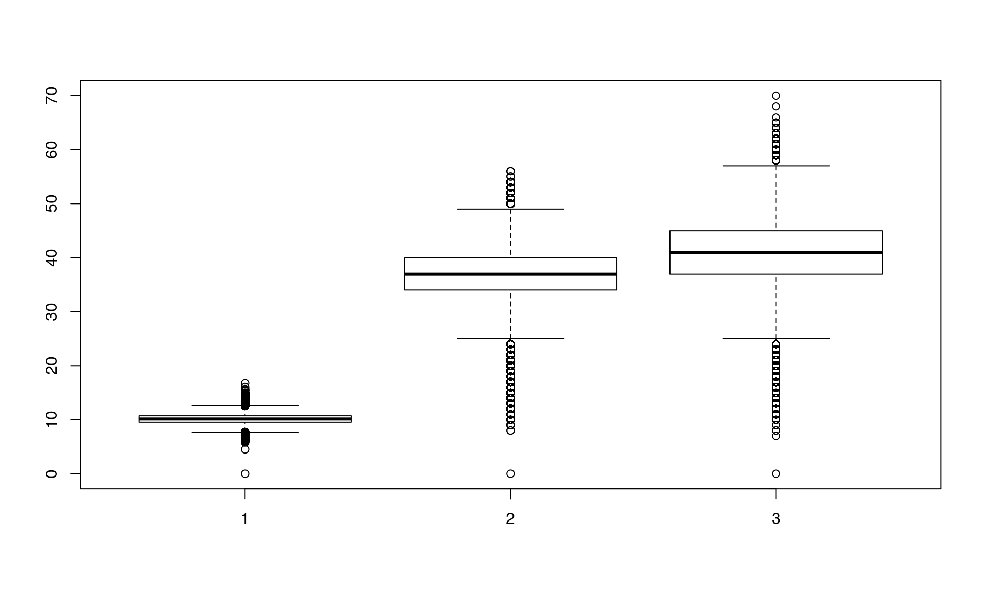
boxplot(distgenEUCL, distgenDIFF, distgenDISS)

The number of allelic differences between two individuals is a different measure from euclidean distance or number of locus differences between two individuals.

Conclusion

What did we learn today?

In this vignette, we explore different measures of individual genetic distances. It is important to investigate the different options of each command. Missing data can be handled in different ways.

What is next?

These individuals genetic distances can then be used in analyses such as Mantel tests to test for isolation by distance, more complex analyses in landscape genetics to test for resistance by distance, cluster analysis, or spatial networks.

Contributors

Stéphanie Manel
Zhian Kamvar (minor edits)

Session Information

This shows us useful information for reproducibility. Of particular importance are the versions of R and the packages used to create this workflow. It is considered good practice to record this information with every analysis.

options(width = 100)
devtools::session_info()

## ─ Session info ───────────────────────────────────────────────────────────────────────────────────
##  setting  value                       
##  version  R version 3.6.1 (2019-07-05)
##  os       Debian GNU/Linux 9 (stretch)
##  system   x86_64, linux-gnu           
##  ui       X11                         
##  language (EN)                        
##  collate  en_US.UTF-8                 
##  ctype    en_US.UTF-8                 
##  tz       Etc/UTC                     
##  date     2019-09-16                  
## 
## ─ Packages ───────────────────────────────────────────────────────────────────────────────────────
##  package     * version  date       lib source        
##  ade4        * 1.7-13   2018-08-31 [1] CRAN (R 3.6.1)
##  adegenet    * 2.1.1    2018-02-02 [1] CRAN (R 3.6.1)
##  ape         * 5.3      2019-03-17 [1] CRAN (R 3.6.1)
##  assertthat    0.2.1    2019-03-21 [1] CRAN (R 3.6.1)
##  backports     1.1.4    2019-04-10 [1] CRAN (R 3.6.1)
##  boot          1.3-22   2019-04-02 [2] CRAN (R 3.6.1)
##  callr         3.3.1    2019-07-18 [1] CRAN (R 3.6.1)
##  class         7.3-15   2019-01-01 [2] CRAN (R 3.6.1)
##  classInt      0.4-1    2019-08-06 [1] CRAN (R 3.6.1)
##  cli           1.1.0    2019-03-19 [1] CRAN (R 3.6.1)
##  cluster       2.1.0    2019-06-19 [2] CRAN (R 3.6.1)
##  coda          0.19-3   2019-07-05 [1] CRAN (R 3.6.1)
##  colorspace    1.4-1    2019-03-18 [1] CRAN (R 3.6.1)
##  crayon        1.3.4    2017-09-16 [1] CRAN (R 3.6.1)
##  DBI           1.0.0    2018-05-02 [1] CRAN (R 3.6.1)
##  deldir        0.1-23   2019-07-31 [1] CRAN (R 3.6.1)
##  desc          1.2.0    2018-05-01 [1] CRAN (R 3.6.1)
##  devtools      2.2.0    2019-09-07 [1] CRAN (R 3.6.1)
##  digest        0.6.20   2019-07-04 [1] CRAN (R 3.6.1)
##  dplyr         0.8.3    2019-07-04 [1] CRAN (R 3.6.1)
##  DT            0.8      2019-08-07 [1] CRAN (R 3.6.1)
##  e1071         1.7-2    2019-06-05 [1] CRAN (R 3.6.1)
##  ellipsis      0.2.0.1  2019-07-02 [1] CRAN (R 3.6.1)
##  evaluate      0.14     2019-05-28 [1] CRAN (R 3.6.1)
##  expm          0.999-4  2019-03-21 [1] CRAN (R 3.6.1)
##  fastmatch     1.1-0    2017-01-28 [1] CRAN (R 3.6.1)
##  fs            1.3.1    2019-05-06 [1] CRAN (R 3.6.1)
##  gdata         2.18.0   2017-06-06 [1] CRAN (R 3.6.1)
##  ggplot2       3.2.1    2019-08-10 [1] CRAN (R 3.6.1)
##  glue          1.3.1    2019-03-12 [1] CRAN (R 3.6.1)
##  gmodels       2.18.1   2018-06-25 [1] CRAN (R 3.6.1)
##  gtable        0.3.0    2019-03-25 [1] CRAN (R 3.6.1)
##  gtools        3.8.1    2018-06-26 [1] CRAN (R 3.6.1)
##  htmltools     0.3.6    2017-04-28 [1] CRAN (R 3.6.1)
##  htmlwidgets   1.3      2018-09-30 [1] CRAN (R 3.6.1)
##  httpuv        1.5.2    2019-09-11 [1] CRAN (R 3.6.1)
##  igraph        1.2.4.1  2019-04-22 [1] CRAN (R 3.6.1)
##  KernSmooth    2.23-15  2015-06-29 [2] CRAN (R 3.6.1)
##  knitr         1.24     2019-08-08 [1] CRAN (R 3.6.1)
##  later         0.8.0    2019-02-11 [1] CRAN (R 3.6.1)
##  lattice       0.20-38  2018-11-04 [2] CRAN (R 3.6.1)
##  lazyeval      0.2.2    2019-03-15 [1] CRAN (R 3.6.1)
##  LearnBayes    2.15.1   2018-03-18 [1] CRAN (R 3.6.1)
##  magrittr      1.5      2014-11-22 [1] CRAN (R 3.6.1)
##  MASS          7.3-51.4 2019-03-31 [2] CRAN (R 3.6.1)
##  Matrix        1.2-17   2019-03-22 [2] CRAN (R 3.6.1)
##  memoise       1.1.0    2017-04-21 [1] CRAN (R 3.6.1)
##  mgcv          1.8-28   2019-03-21 [2] CRAN (R 3.6.1)
##  mime          0.7      2019-06-11 [1] CRAN (R 3.6.1)
##  munsell       0.5.0    2018-06-12 [1] CRAN (R 3.6.1)
##  nlme          3.1-140  2019-05-12 [2] CRAN (R 3.6.1)
##  pegas       * 0.11     2018-07-09 [1] CRAN (R 3.6.1)
##  permute       0.9-5    2019-03-12 [1] CRAN (R 3.6.1)
##  phangorn      2.5.5    2019-06-19 [1] CRAN (R 3.6.1)
##  pillar        1.4.2    2019-06-29 [1] CRAN (R 3.6.1)
##  pkgbuild      1.0.5    2019-08-26 [1] CRAN (R 3.6.1)
##  pkgconfig     2.0.2    2018-08-16 [1] CRAN (R 3.6.1)
##  pkgload       1.0.2    2018-10-29 [1] CRAN (R 3.6.1)
##  plyr          1.8.4    2016-06-08 [1] CRAN (R 3.6.1)
##  polysat       1.7-4    2019-03-06 [1] CRAN (R 3.6.1)
##  poppr       * 2.8.3    2019-06-18 [1] CRAN (R 3.6.1)
##  prettyunits   1.0.2    2015-07-13 [1] CRAN (R 3.6.1)
##  processx      3.4.1    2019-07-18 [1] CRAN (R 3.6.1)
##  promises      1.0.1    2018-04-13 [1] CRAN (R 3.6.1)
##  ps            1.3.0    2018-12-21 [1] CRAN (R 3.6.1)
##  purrr         0.3.2    2019-03-15 [1] CRAN (R 3.6.1)
##  quadprog      1.5-7    2019-05-06 [1] CRAN (R 3.6.1)
##  R6            2.4.0    2019-02-14 [1] CRAN (R 3.6.1)
##  Rcpp          1.0.2    2019-07-25 [1] CRAN (R 3.6.1)
##  remotes       2.1.0    2019-06-24 [1] CRAN (R 3.6.1)
##  reshape2      1.4.3    2017-12-11 [1] CRAN (R 3.6.1)
##  rlang         0.4.0    2019-06-25 [1] CRAN (R 3.6.1)
##  rmarkdown     1.15     2019-08-21 [1] CRAN (R 3.6.1)
##  rprojroot     1.3-2    2018-01-03 [1] CRAN (R 3.6.1)
##  scales        1.0.0    2018-08-09 [1] CRAN (R 3.6.1)
##  seqinr        3.6-1    2019-09-07 [1] CRAN (R 3.6.1)
##  sessioninfo   1.1.1    2018-11-05 [1] CRAN (R 3.6.1)
##  sf            0.7-7    2019-07-24 [1] CRAN (R 3.6.1)
##  shiny         1.3.2    2019-04-22 [1] CRAN (R 3.6.1)
##  sp            1.3-1    2018-06-05 [1] CRAN (R 3.6.1)
##  spData        0.3.0    2019-01-07 [1] CRAN (R 3.6.1)
##  spdep         1.1-2    2019-04-05 [1] CRAN (R 3.6.1)
##  stringi       1.4.3    2019-03-12 [1] CRAN (R 3.6.1)
##  stringr       1.4.0    2019-02-10 [1] CRAN (R 3.6.1)
##  testthat      2.2.1    2019-07-25 [1] CRAN (R 3.6.1)
##  tibble        2.1.3    2019-06-06 [1] CRAN (R 3.6.1)
##  tidyselect    0.2.5    2018-10-11 [1] CRAN (R 3.6.1)
##  units         0.6-4    2019-08-22 [1] CRAN (R 3.6.1)
##  usethis       1.5.1    2019-07-04 [1] CRAN (R 3.6.1)
##  vegan         2.5-6    2019-09-01 [1] CRAN (R 3.6.1)
##  withr         2.1.2    2018-03-15 [1] CRAN (R 3.6.1)
##  xfun          0.9      2019-08-21 [1] CRAN (R 3.6.1)
##  xtable        1.8-4    2019-04-21 [1] CRAN (R 3.6.1)
##  yaml          2.2.0    2018-07-25 [1] CRAN (R 3.6.1)
## 
## [1] /usr/local/lib/R/site-library
## [2] /usr/local/lib/R/library

Individual Based Genetic Distance for SNP Data